Microeconomics
Microeconomics is concerned with how much a single business should produce (not covered here) and how goods and services for one specific market might behave. When determining the behavior of a particular market, microeconomics makes several assumptions:
- There is a vast quantity of suppliers with relatively equal production capacity so no one firm is able to have an effect on the total amount being produced and therefore will have no ability to affect the price.
- There is a vast quantity of consumers with relatively equal purchasing capacity so no one consumer is able to have an effect on the total amount being bought and therefore will have no ability to affect the price.
- Free competition between all producers and consumers results in prices finding their lowest equilibrium points.
- Products in a given market can not be differentiated from one another.
- When a change is made in the economy, all other things are held equal.
Microeconomics and even economics in general is based on the idea that finite resources must be allocated in different configurations to maximize output.
Scarcity and Production Possibilities
For a more in depth discussion of microeconomics, we start first with the idea of scarcity. There are not an infinite number of resources to be had in any economy. Therefore, competition will arise for use of the scarce resources that are available. Resources in an economy can be used to produce goods and bads. Goods are things people are willing to trade for like cars and dental services. Bads are things that people do no want such as litter or smog. Bads will become important again in another essay. For now it is enough to know they exist. Resources do not have to be just materials like copper, water, or bananas. Resources can be things like available labor, or aggregate ambition (the total drive with a population to be productive). However, not all resources are made equal, some are worth more than others, so some rationing device is normally used for distribution of said resources.
Resources are also not perfectly adaptable. This means that shifting from production of apples to oranges will not yield exactly one less apple and one more orange. There are diminishing returns for resource reallocation. These diminishing returns bring us to the idea of a Production Possibilities Frontier model in a simple two good economy.
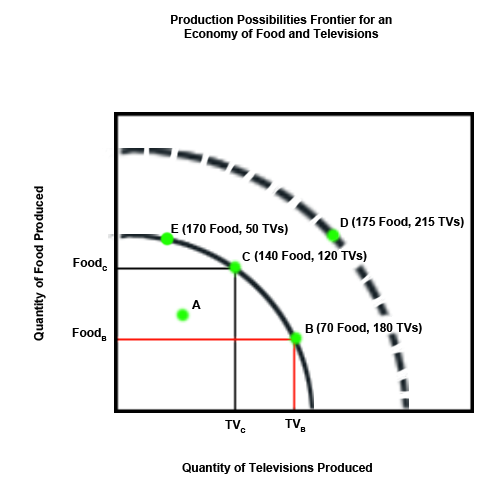
Imagine an economy where the two goods produced are televisions and food. A general case for a Production Possibilities Frontier (PPF) would look something like a quarter circle drawn onto a graph with the x axis labeled as the output of televisions for the economy and the y axis labeled as the output for food (example). The quarter circle curve represents the maximum output of all resources in the economy. Any level of production that lies on or inside the curve is possible and any point outside the curve is not possible to produce at because such a level of production would require more resources than are currently available.

If we take a look at the example, points A, B, C, and E are possible and point D is not. Point A is an inefficient level of production because not all resources are being utilized. Point A represents inefficiency in microeconomics and unemployment in macroeconomics (unemployment will be discussed later in macroeconomics). Points B and C are efficient because all available resources in the economy are being used. To an economist, point C is not necessarily better than point B or vice versa. Economists draw the distinction between points B and C in terms of advantages and opportunity costs. The advantage of producing at point B rather than point C is the extra amount of televisions produced (calculated by TVB - TVC). The opportunity cost of producing at point B instead of point C is the amount of food that is forgone (calculated as Food C - Food B). The advantage of producing at point C rather than point B is the extra amount of food produced (calculated by Food C - Food B). The opportunity cost of producing at point C instead of point B is the amount of televisions that are forgone (calculated as TVB - TVC). Also from the example we can see that it becomes more and more expensive in terms of food when trying to increase production of televisions and vice versa. This phenomenon is due to resources being specialized and not perfectly adaptable. For example, it is more difficult to make televisions with the foregone fertilizer from less food production than it is from a shift in the labor force.
The only way to produce at point D is to have economic growth that provides more resources. This growth can take the form of having more children to increase the labor pool, acquiring more land to grow more food, or acquiring more mineral mines to increase the quantity of inputs of production for televisions.
To put it succinctly, resources in an economy are limited and specialized. This creates a need to balance allocation of the available resources with regard to the needs of the economy. A production possibilities frontier curve is a visual representation of all of the possible output combinations possible for a given set of resources and can be used to visualize the idea of diminishing returns for specialized resources. These principles are used later in understanding the long run aggregate supply curve of macroeconomics.
Supply and Demand
From the idea of scarcity, we move on to the principles of microeconomic supply (the amount of a good or service produced for a market) and demand (the amount of a good or service desired in a market). In this model there are a large enough number of producers and consumers of a given good so that no one entity (business or consumer) has the ability to affect price in any meaningful manner. The model only represents the supply and/or demand for a particular good or type of goods in a specific time period.
Demand
First, we will consider demand. In almost every case, as the price of good increases, the quantity demanded decreases. It happens often enough that economists call it the law of demand. This phenomenon can be explained through what is known as the substitution effect. The substitution effect is the idea that people substitute relatively lower priced goods for relatively higher priced goods. An example of this would be the cereal market. If the price for name brand cereals rises, people will look for lower priced substitutes of those cereals. We expect that at least some people will be able to find an acceptable substitute. Therefore, we expect the quantity of name brand cereals purchased to decrease when the price for those cereals rises. From this we can gather that a simple demand curve would look something like a downward sloping line. As price increases, quantity demanded decreases as in this example.
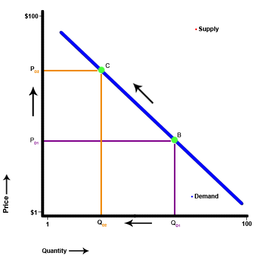
(Those of you who are math oriented, may notice that for some reason economists placed the independent variable on the vertical axis and the dependant variable on the horizontal axis. I have no idea why economists do this, but it does not change the slope, direction of the curves, or how they interact with each other, so I will stick with convention)
It is important to note that a change in the price of a good, changes only the quantity demanded not the total demand (desirability). To be put another way, the price of a good affects the quantity demanded for that good but does not change the number of people willing to buy at a given price so there is movement along the original curve.
Supply
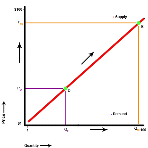
Conversely, as the price of a good increases, the quantity supplied also increases. Higher prices are an incentive to suppliers to produce more of a good. This incentive takes the form of higher profits.
�
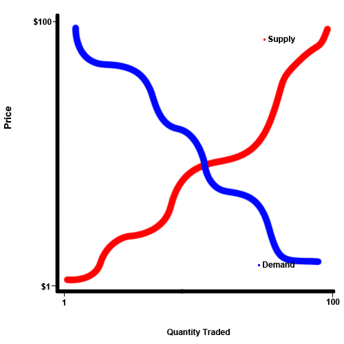
Realistically, supply and demand curves would not be straight lines but would be varied and nuanced. At prices that approached certain psychological barriers (under $10, under $1 per unit, etc.), there may be little movement in the quantity demanded until that threshold is crossed and then a sudden change in the quantity demanded occurs. Supply may have a similar shape but has its psychological barriers at different points that represent certain profit percentages (10% margin, 25% margin, etc.). However, the exact shape of the curves does not change their overall behavior or how they interact with each other, just where the exact equilibrium price and quantity are. So for our general understanding purposes, simple sloped lines will suffice.
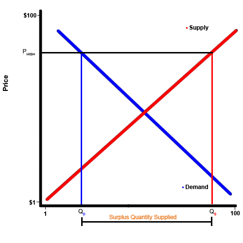
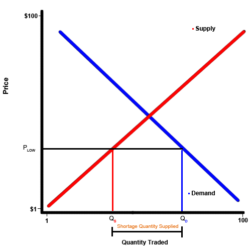
If the quantity of a good supplied in a market is greater than the quantity demanded, then a surplus or excess supply exists. If the quantity demanded is greater than the quantity supplied, then a shortage or excess demand exists.
Surplus
In the case of a surplus, the additional supply is a signal for the price to drop in order to increase the number of trades or sales. In reality, this would look like hundreds of basketballs sitting on retail shelves selling for $150. Since the basketballs are not selling at this price point and the available stock is very large, there is an indication that the price should be lowered in order to affect more sales. As the price decreases there will be more basketballs demanded and fewer supplied. This movement along the supply and demand curves continues until the surplus is eliminated.
Shortage
In the case of a shortage, the pressure on the price is the opposite. The additional demand, or lack of supply, is a signal for the price to increase. People will respond to the shortage by offering to buy or sell at a higher price. Like in the case of the surplus, this produces movement on both the supply and demand curves until the shortage disappears.
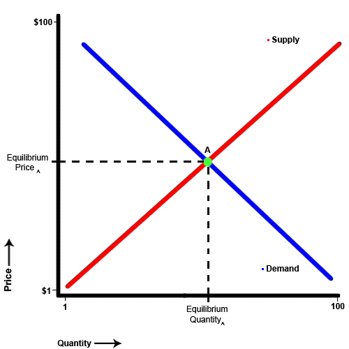
Market Equilibrium
Once there is no longer a shortage or a surplus, we say that the market has reached equilibrium. Equilibrium occurs when the quantity supplied equals the quantity demanded. There is only one equilibrium for a given time period. Since there is neither a surplus nor a shortage, there are no signals for the price to change in either direction.
Demand Shifts
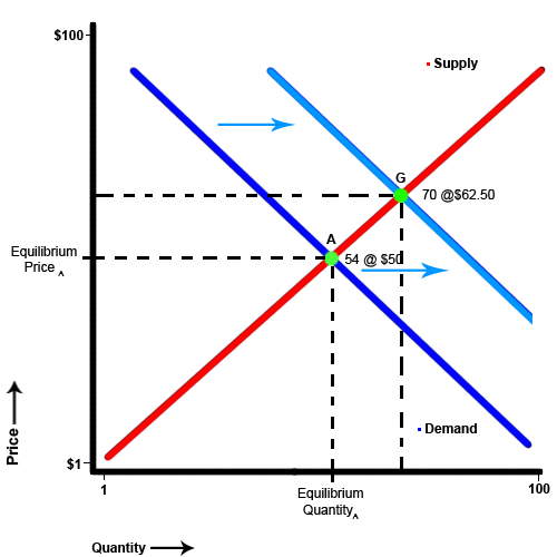
Equilibriums exist for a particular time period and do not last indefinitely. This happens because market forces move the equilibrium point. In the case of demand, there are six major factors that can shift the demand curve: income, preferences, prices of substitutes, prices of complements, number of buyers, and price expectations. These factors create a different quantity demanded for every price point. The general shape of the curve is maintained but the entire curve shifts. For example, instead of 54 people demanding a good at $50 there are now 90 people that demand that good at $50.
Income Changes
If the income of buyers increases, buyers are more willing to buy the good at higher prices. For example, if there are 54 people willing to buy a silver watch for $50 normally and then the incomes of perspective buyers increases, there will be more people willing to buy the watches at a higher price. This put upward pressure on the price and since the price is rising, suppliers are willing so supply more silver watches and the market arrives at a new equilibrium with 70 buyers willing to purchase silver watches at a price of $62.50. Alternatively, if the income of buyers decreases, all buyers are less willing to buy at the current price and demand for the market decreases.
Prices of Substitutes
Prices of substitutes affect the demand curve in a similar manner. Substitutes are goods that can be substituted for one another without a large loss in quality. Many people will use Coca-Cola and Pepsi as an example of substitute goods; earlier we considered name brand cereal and off brand cereal. Still, a better example would be two equal but separate brands of strawberry jelly. If the price of Brand A increases for some reason, there will be an increase in the demand for Brand B as people shift towards using the cheaper substitute.
Prices of Complementary Goods
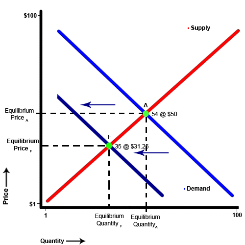
Complementary goods are those that are consumed together. Examples of this include tennis rackets and tennis balls, bread and peanut butter, and milk and cereal. If there is a rise in the price of a good then demand for the complement decreases and vice versa. For instance, in increase in the price of tennis rackets will cause a decrease in the demand for tennis balls. For instance, an increase in price for tennis rackets causes a lower quantity of tennis rackets to be purchased. Since nearly everyone buying a tennis racket will need to purchase tennis balls, this change in the quantity of tennis rackets demanded leads to a complete shift in the demand for tennis balls. We can see that this shift leads to fewer people demanding tennis balls at every price point. The lower demand puts downward pressure on the price. At a lower price there are fewer suppliers willing to sell tennis balls. In our example the scenario resolves itself to a new equilibrium of 35 people willing to pay $3.15 for a can of tennis balls down from 54 people willing to pay $5 for a can of tennis balls.
Number of Buyers
The number of buyers affects the entire demand curve by adding more or removing people willing to buy a good at every price point.
Price Expectations
Finally, expectations of future prices for a good shift the demand curve for a it by compelling people to by the good sooner if the expectation is that prices will be higher and compelling people to buy the good later if the expectation is that prices will be lower.
Supply Shifts
For supply, there are seven major factors that can cause a shift in supply: prices of relevant resources, technology, number of sellers, sellers price expectations, taxes, subsidies, and government restrictions. These factors create a different quantity of a good that sellers are willing and able to supply at every price point. Similar to how the demand curve shifts, the supply curve shifts in response to these factors.
Prices of Relevant Resources
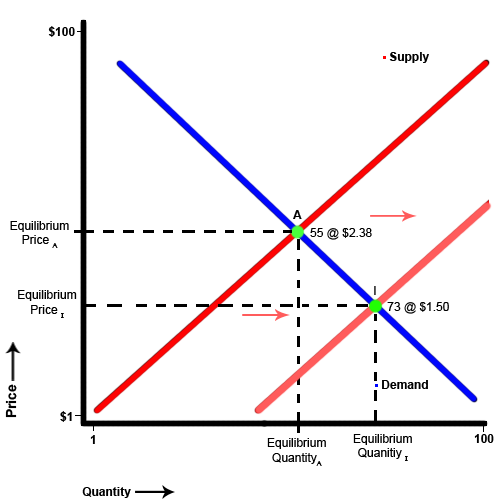
If there is a decrease in the price of a relevant resource, like the price of wheat decreasing when looking at the market for bread, then supply increases and the supply curve shifts to the left. Since the price of wheat (an input) is lower, it is now easier for suppliers to make their expected profits. This entices other suppliers to enter the market and current suppliers to make more bread. This shift indicates that there are more suppliers willing to sell at every price point. The increased willingness to sell puts downward pressure on prices which increases the quantity demanded. In our example, the equilibrium shifted from 55 loaves being sold at $2.38 each to 73 loaves being sold for a mere $1.50 each.
Number of Sellers
Like the demand curve, the number of sellers can shift the supply curve. If the number of sellers in a market decreases, there will be fewer suppliers willing to sell at every given price point. In this case, the supply decreases and the supply curve shifts left. This phenomenon puts upward pressure on prices. The new equilibrium results in higher prices and fewer trades.
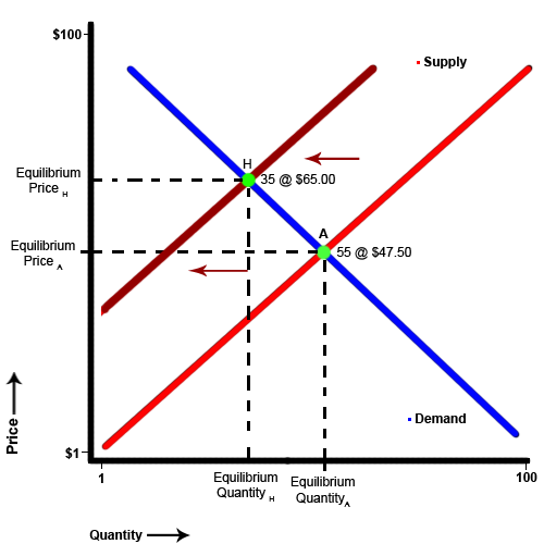
As an example, we can examine what happens when floods in Thailand destroy factories that create hard drives. Since there are fewer suppliers, there are fewer suppliers willing to sell at every given price point. Therefore, the supply curve shifts left. The equilibrium shifts from 55 hard drives being sold for $47.50 to 35 hard drives being sold for $65.00.
Price Expectations
Furthermore, sellers price expectations also affect the behavior of the supply curve. If suppliers expect prices to fall in the future, then they all act to sell quickly before the price falls. This action takes the form of lowering prices. Since all sellers in the market are taking this action, the entire curve shifts.
Taxes and Subsidies
As for taxes and subsidies, they act much in the same way as prices of relevant resources or inputs. Some taxes increase the per-unit cost of producing a good. If there is a $500 tax placed on each car manufactured, there will be fewer suppliers willing to sell at every price point than if there had been no tax so the supply curve shits leftward. Conversely, if the tax is lowered to $250 per car produced, there will be more suppliers willing to sell at every price point than previously so the supply curve will shift to the right.
Subsidies work in the opposite manner. Suppose the government pays suppliers $5 for every bushel of strawberries they produce. Because of the higher selling price point, there is going to be a greater quantity supplied at every price point which shifts the supply curve to the right. If the subsidy is removed or lowered, the supply curve then shifts to the left.
Government Restrictions
Sometimes governments act to increase or reduce supply through means other than taxes and subsidies. One way to accomplish this is through import quotas. If, for example, the United States sets an import quota on Korean automobiles, only a certain quantity may enter into the United States. This action limits supply and shifts the supply curve leftward (supply decreases). Removing said limit or increasing the limit would allow the supply curve to shift to the right (supply increases). Licensure is a method governments can use to limit the supply of certain types of labor. It may not be the intention of limiting the supply, but by requiring engineers to get licenses to operate, the government decreases the number of engineers supplied and thereby shifts the supply curve to the left (supply decreases).
Technology
Finally, technology as it pertains to economics does not necessarily indicate computers and robots. Technology is the body of skills and knowledge used in changing resources into goods. As an example, the cotton gin is used to separate cotton fibers from seeds or irrigation is used to water crops instead of just waiting for rain. Advancement in technology lowers the per-unit cost of production. Lower per-unit costs mean more profits are able to be made and incentivize suppliers to produce more at every price point and therefore shift the supply curve to the right. Regressions in technology happen most often in locations hit by natural disaster. While the knowledge and skills have not been lost to society as a whole, the affected area will for a short time behave as if there had been a regression in technology (loss of power, loss of running water).
To summarize, in microeconomics various combinations of scares resources are used to determine the maximum output for an economy. Changes in the price of a good or service change the quantity supplied and the quantity demanded but do not affect total supply or total demand. Total demand can be affected by consumer income, preferences, prices of substitutes, prices of complements, number of buyers, and consumer price expectations. Total supply can be affected by prices of relevant resources, technology, number of sellers, sellers' price expectations, taxes, subsidies, and government restrictions.
Microeconomics is a great way to introduce concepts for economics. However, the assumptions of vast pools of producers that cannot have an effect on price and undifferentiated products are unrealistic. Because product differentiation does exist, some firms are able to sell more of a particular good. This allows them to make more money and invest in expansion. With expansion comes more market share. If economies of scale exist for a particular market (the average cost of producing one more unit falls as a firm produces more), then the eventual outcome is either monopoly (one firm controlling all or most of the production for a particular market) or oligopoly (few firms controlling most of the production for a market).
Monopoly and oligopoly are inefficient because the competition that would normally drive prices to their lowest equilibrium point does not exist. Why competition does not happen under oligopoly even if collusion is illegal is explained in game theory which is a topic for another day.
Because of these unintended outcomes and unrealistic assumptions, we turn to macroeconomics for ideas on how to manipulate the economy as a whole.
Macroeconomics
Macroeconomics is chiefly concerned with raising the quality of life of all individuals in an economy. The major mechanism used to address this concern is trade. Therefore, in understanding and manipulating trade, there are three important goals in macroeconomics:
1. Price Stability
2. Sustained economic growth
3. Low unemployment
To achieve these goals, economists conduct what is termed stabilization policy. First, economists measure price levels of all goods and services in the economy, the growth rate of output of goods and services, and the unemployment rate. Then economists compare these measurements to previous measurements to identify the direction and magnitude of any changes. Finally, if the results of comparison show that the goals of prices stability, sustained economic growth, and low unemployment are not being met, economists use different tools and techniques to stabilize the economy to help meet those goals.
Measurements
Price Level
Price level is the weighted average for all goods and services in the economy. There are tens of millions of goods and services produced in the United States annually. These goods and services can be broken up into four distinct areas.
- Goods and services bought by the government.
- Goods and services bought by businesses (investment).
- Goods and services bought by consumers.
- Goods and services entering world trade (exports).
Consumer Price Index
Consumer spending is by far the largest of these categories and is the one that most greatly affects the day-to-day lives of our citizens. To that end the government uses a measure called the Consumer Price Index (CPI) to estimate the price level for a given time period. The CPI takes a weighted average of a basket of 90,0000 goods each month. This weighted average can then be compared to previous months or years to determine what changes there have been to the consumer price level. The CPI is not perfect. It is a good indicator, however it sometimes tends to overstate inflation because it fails to take into account new goods which may have rapidly fallen in price.
Gross Domestic Product Implicit Deflator
A second measure used to determine price level is the Gross Domestic Product Implicit Deflator (GDP deflator). The GDP deflator is similar to the CPI but instead of measuring just goods and services purchased by households, it also measures the prices of goods and services purchased by government, businesses, and those entering world trade.
By comparing the CPI or GDP deflator to different years economists can see whether or not the economy is experiencing inflation, disinflation, deflation, or price stability. If either of the indicators is increasing, the economy is experiencing inflation. If they are increasing but more slowly than they had been previously, the economy is experiencing disinflation. If price levels are decreasing, then the economy is experiencing deflation. If there is no change, the economy has price stability.
Inflation
Inflation means that tomorrow's dollar will be worth less than today's dollar. The magnitude of this effect is very important. If inflation is very high, (above 10% anually) then people on fixed incomes, people who save much of their money, and lenders are negatively impacted. The incentive under high inflation is to spend as quickly as possible to avoid further loss in value of your money. Unfortunately, the increased spending only serves to further drive up prices and exacerbate the inflation. Fortunately, central banks and governments have good tools they can use to combat inflation. Also, relatively low inflation does not have as great an impact, and as long as wages are outpacing inflation there is no problem.
Inflation causes another problem and that is one of comparison. Because of inflation $100 in 1980 bought more goods than $100 in 2005. The CPI or GDP deflator can be used to normalize those numbers so they can be compared equivocally. So, $100 in 1980 would be equal to $236 in 2005. When economists compare terms like this, they us the term real. So real wages are those that have been adjusted for inflation. For example, a person who made $20,000 a year in 1980 and made $30,000 a year in 1995 had their nominal wages increase by $10,000 per year. However, adjusted for inflation, the persons real wages went from $20,000 1980 dollars to $16,274 1980 dollars in 1995. Put another way, making $30,000 in 1995 was the same as making $16,274 in 1980. In this scenario, the person's real income fell.
Deflation
Deflations means tomorrow's dollar with be worth more than today's dollar. Deflation is very dangerous because it does not take a great magnitude of it to make self fulfilling spiral downward. Deflation incentivizes people to wait until later to spend. This means people save in much greater numbers. The reduced spending in the economy drives down prices further and more people save their money instead of spending. It is important to understand that the entire economy is driven by spending. So the economy actually shrinks, as does the money supply. With less supply of money, each dollar becomes more valuable. Even worse, there are no proven methods to combat or even control deflation (My argument is that you would need to use drastic measures that would normally spark hyper inflation for a very short time, but that is for another day).
Unemployment
To measure unemployment, the population has to be separated into two groups: those in the labor force and those not in the labor force. In the United States, we consider anyone age 16 or older who has worked for pay or profit during the survey period, anyone who has done 15 hours of unpaid labor for a family operated enterprise, and anyone that has a regular job but has been temporarily absent due to illness, strike, vacation, or other personal reasons as employed. We consider those who are actively seeking a job or are waiting to be called back from a temporary lay off and are available to work unemployed. Anyone under the age of 16, anyone that is institutionalized, anyone who is a member of the armed forces on active duty, and anyone else who is not employed or unemployed is not in the labor force. The unemployment rate is the number of people who are unemployed versus the total number of people in the labor force. The way we measure unemployment in the United States tends to understate the unemployment rate a bit. The reason for this is that there are people who have not been looking for work recently but would take a job if one were offered. We consider these people out of the labor force but their existence can be an indicator of the strength or weakness of an economy. Furthermore, in this model we don't capture people who are employed but have wages that are far lower than what the market rate for their skills is. We call these people underemployed, but they do not affect the unemployment rate.
Unemployment can be broken down into three types: frictional, structural, and cyclical.
Frictional Unemployment
Frictional unemployment is when people with transferrable skills leave some jobs and move to others. Consider secretaries or computer programmers moving from one firm to another as demand for their products changes and some are let go and others are hired.
Structural Unemployment
Structural unemployment is caused by changes in the structure to the economy that cause displaced workers to not have transferrable skills. For example, stage coach drivers could not immediately become automobile drivers when their craft became obsolete.
Cyclical Unemployment
Cyclical unemployment is total unemployment minus structural and frictional unemployment. Cyclical unemployment occurs when there is not enough spending in the economy.
Economists expect that there will always be some structural and frictional unemployment. These two types of unemployment add together to become what is considered the natural unemployment rate. In the United States this figure is estimated to be 3-4%. At that point the country is said to be at full employment. Full employment occurs when there is no longer any cyclical unemployment.
Economic Growth
Economic growth is most commonly measured by the Gross Domestic Product (GDP). The GDP is the total market value of all final goods and services purchased annually within a country's borders. Real GDP is GDP that has been adjusted for inflation. GDP is a very good measurement for how an economy is doing overall but it does have some limitations. For instance, if there is a population boom, or if one particular segment of the population becomes incredibly more productive, real GDP may increase, but the lives of many of the people in the economy may not have changed, or worse, they may have deteriorated. To compensate for this, one can look at real GDP per capita which is each person's share of the GDP for a country. However, even with this compensation, the GDP measure still fails to capture things like leisure time, friendship, pollution, crime, happiness, etc and these other factors also influence quality of life.
There are several factors that influence growth rates: Level of economic freedom (freedom to produce and consume without government quotas), property rights structure (copyright and patent laws), trade policies(enacting tariffs or trade quotas) , technological advance (using different methods to produce more with the same resources), capital (land or equipment used for business), human capital (knowledge skills and abilities of the workforce), population levels, and natural resources. These factors can really be distilled to GDP being equal to the amount of output the average worker can produce in an hour multiplied by the average number of hours in the work week, multiplied by the labor force participation rate, multiplied by the population.
GDP = (productivity) * (average work week hours) * (labor force participation rate) * (population)
Increasing any of these four factors can increase the GDP. Population growth may lead to more output, the result may not be higher per capita GDP. The labor force participation rate has an upper limit of 100% and there is also an upper limit of 168 hours available to work in a week. Therefore, the way to continually increase output is to increase productivity.
There are three ways to increase productivity: increase capital stock (resources), increase human capital (the knowledge and skills possessed by workers), and achieve technological progress. (The latter two seems to be heavily influenced by education, but that is an article for another day.)
To summarize, macroeconomics is concerned with increasing the quality of life of individuals in an economy through trade. Economists try to achieve this through price level stability, sustained economic growth, and low unemployment. Macroeconomists use the Consumer Price Index (CPI) and the Gross Domestic Product Deflator (GDP Deflator) to measure the price level in an economy. If the price level is rising, the economy is said to be experiencing, inflation. If the price level is decreasing, the economy is experiencing deflation; if the price level is not changing, the economy is experiencing price level stability. Frictional and structural unemployment in an economy are natural and small quantities of either are not harmful to an economy. Cyclical unemployment is caused by a lack of spending in an economy and is an indicator for the health of an economy. Economic growth is best measured by changes in the Real GDP per capita. With these measurements economists the consider macroeconomic supply and demand to evaluate causes for economic events and possible corrective actions.
Macroeconomic Supply and Demand
As with microeconomics, macroeconomics also deals with supply and demand curves. The difference is that instead of concentrating on one market, macroeconomics looks at all the markets combined. With this model economists can gauge the impact policy decisions have on price level, economic output, and unemployment.
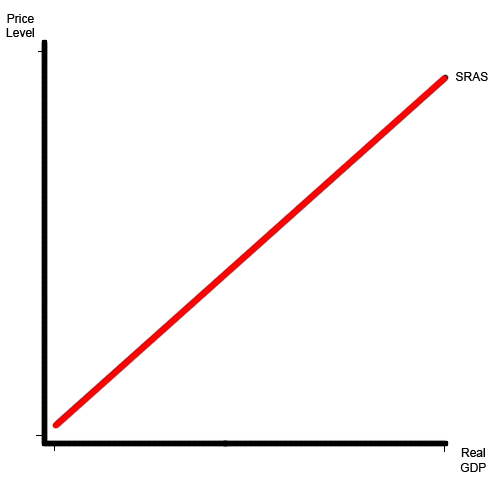
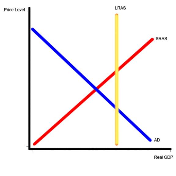
Short Run Aggregate Supply
Aggregate supply is the quantity of real GDP supplied at different price levels. In the short run, there is a positive relationship between price level and the quantity of GDP supplied. There are three main factors that can shift the short run aggregate supply curve (SRAS): a change in productivity, a change in the price of inputs (wages, fuel costs, etc.), and supply shocks (a blizzard wipes out the orange crop in Florida, a sharp decrease in the amount of oil imported to the United States because of an international oil embargo).
Aggregate Demand
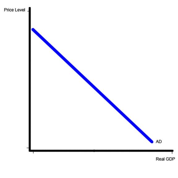
Aggregate Demand is the quantity of real GDP demanded by households, businesses, government, and foreigners at different price levels. As with demand in microeconomics, there is an inverse relationship between the price level and the quantity or real GDP demanded.
There are four components to calculating aggregate demand: consumption, investment, government spending, and net exports. Aggregate demand can be represented by the equation below.
Aggregate Demand = Consumption + Investment + Government spending + (EXports - IMports)
There are eleven major factors that can shift the aggregate demand curve:
Consumption
1. A change in wealth (higher or lower home values, or higher or lower values for items that people use to hold money like cars or paintings). A in increase in wealth shifts the curve to the right a decrease in wealth shifts the curve to the left.
2. Consumers' expectations of higher or lower future prices (People expect the inflation rate to be higher or lower or expect imports to be more or less expensive soon.). An expectation of higher prices gives everyone an incentive to make purchases sooner rather than later. The increase in demand, without a corresponding increase in supply raises the price level. On the other hand, if consumers expect lower prices, the aggregate demand curve shifts to the left.
3. Consumers' expectations of higher or lower incomes. Expectations of higher incomes shifts aggregate demand to the right and expectations of lower incomes shifts aggregate demand to the left. This is because people are likely to spend increased income before they recieve it and likely to begin saving more income if there is a likelyhood of lower wages.
4. A change in interest rates. A decrease in interest rates makes items that people normally take out loans for less expensive and also creates less incentive to save since the money saved will not earn as much as it previously had. These factors combine to increase aggregate demand and shift the curve to the right. An increase in interest rates has the opposite effect.
5. A change in personal income taxes. Changing personal income taxes can be viewed as changing incomes. A decrease in personal income taxes is similar to an increase in personal income and will have a similar effect. Not surprisingly, an increase in personal taxes will behave like a decrease in personal income and shift the aggregate demand curve to the left.
Investment
6. Producers' expectations of future sales. If businesses expect to sell more goods in the future then they will be more likely to invest more in the business. The increase in investment spending causes a shift in the aggregate demand curve to the right. If businesses become pessimistic about future sales, they will decrease investment spending and the aggregate demand curve will shift to the left.
7. A change in interest rates. As the interest rate rises the cost of borrowing money for investment projects becomes higher and businesses invest less. As the investment decreases, aggregate demand decreases and the aggregate demand curve shifts leftward. Naturally, a decrease in the interest rate will have the opposite effect and curve will shift to the right.
8. A change in business taxes. Changing business taxes changes businesses' expectations of profitability. Higher business taxes reduces expectations of profits thereby reducing investment spending and shifting aggregate demand to the left. A decrease in business taxes will have the opposite effect of shifting the curve to the right.
Government Purchases
9. A change in government spending. An increase in government spending increases demand for the whole economy and therefore shifts the aggregate demand to the right while a decrease in government spending shifts it to the left.
Net Exports
10. A change in foreign real national income. If the real income of a foreign population increases, then their purchasing power allows them to demand more of our export goods. The increase in the export goods shifts the demand curve to the right. A contrary effect is exhibited when the real income of a foreign populations decreases.
11. A change in the value of the U.S. dollar. If the value of the U.S. dollar decreases with respect to another currency, the foreign country can now buy more U.S. exports because one unit of their currency is now worth more in terms of dollars. This added value to foreign currency allows the U.S. to export more goods and shifts the aggregate demand curve to the right. Alternatively, if the value of the U.S. dollar increases with respect to another currency, the foreign currency is now worth less and can not purchase as much in U.S. goods as it previously had. Such a scenario would lead to fewer U.S. exports and a shift in the aggregate demand curve to the left.
Long Run Aggregate Supply
The long-run aggregate supply curve is a graphical representation of the potential a nation has to produce. Increases or decreases in production based on factors such as quantities of available resources; available technology levels; and governmental regulatory, industrial, and tax policies govern the position of the curve rather than price. While price fluctuations will affect short term supply numbers these price changes will normalize to the equilibrium value, adjusting for misconceptions made in labor value. This is often referred to as the Natural Real GDP and is represented as a vertical line on the Aggregate Supply and Demand graph.
The long run equilibrium is the level of real GDP that the economy produces when wages have adjusted to equilibrium levels and there are no longer any misconceptions on the part of workers in regard to their level of pay when adjusted for inflation.
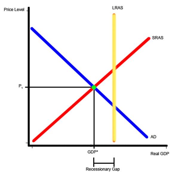
When the level of aggregate demand (AD) is equal to the short run aggregate supply (SRAS), the resultant level of GDP is referred to as the short run equilibrium. When the short run equilibrium is to the left of the long run aggregate supply (LRAS), then the economy is said to be in a recessionary gap. A recessionary gap is characterized by unemployment that is higher than the natural rate of unemployment.
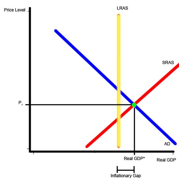
When the short run equilibrium is to the right of the LRAS, the economy is in an inflationary gap. More typically, this is called accelerating inflation meaning that the high level of inflation is sparking more inflation. In this case, unemployment is lower than the natural rate of unemployment.
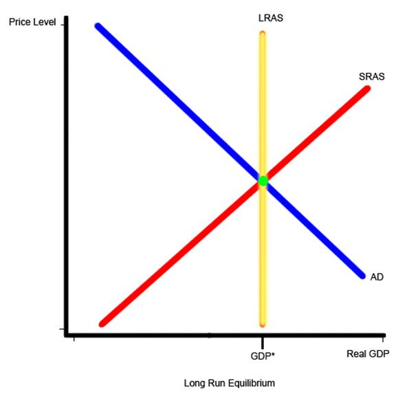
When the short run equilibrium is along the LRAS curve, the economy is in long run equilibrium and unemployment is at the natural rate of unemployment.
In summation, short run aggregate supply (SRAS) is the quantity of real GDP supplied at different price levels in the near term. The SRAS can be affected by a change in productivity, a change in the price of inputs, and supply shocks. Aggregate Demand is the quantity of real GDP demanded by households, businesses, government, and foreigners at different price levels. Aggregate demand can be affected by a change in wealth, income, personal income taxes, business taxes, government spending, the value of the U.S. dollar, or foreign real national incomes; consumers' expectations of future prices and incomes; and producers' expectations of future sales. The long-run aggregate supply curve is a graphical representation of the total production potential a nation has and is price level independent. The various positions of the short run equilibrium with respect to the long run aggregate supply indicate whether the economy is in a recessionary gap, accelerating inflation, or long run equilibrium.
Synopsis
Synoptically, resources in an economy are limited and specialized. This creates a need to balance allocation of the available resources with regard to the needs of the economy. A production possibilities frontier curve is a visual representation of all of the possible output combinations possible for a given set of resources and can be used to visualize the idea of diminishing returns for specialized resources.
In microeconomics various combinations of scarce resources are used to determine the maximum output for an economy. Changes in the price of a good or service change the quantity supplied and the quantity demanded but do not affect total supply or total demand. Total demand can be affected by consumer income, preferences, prices of substitutes, prices of complements, number of buyers, and consumer price expectations. Total supply can be affected by prices of relevant resources, technology, number of sellers, seller price expectations, taxes, subsidies, and government restrictions.
The microeconomic assumptions of vast pools of producers that cannot have an effect on price and undifferentiated products are unrealistic. These unrealistic assumptions eventually lead to either monopoly or oligopoly. Monopoly and oligopoly are inefficient because the competition that would normally drive prices to their lowest equilibrium point does not exist.
Macroeconomics is concerned with increasing the quality of life of individuals in an economy through trade. Economists try to achieve this through price level stability, sustained economic growth, and low unemployment.
Macroeconomists use the Consumer Price Index (CPI) and the Gross Domestic Product Deflator (GDP Deflator) to measure the price level in an economy. If the price level is rising, the economy is said to be experiencing, inflation. If the price level is decreasing, the economy is experiencing deflation; if the price level is not changing, the economy is experiencing price level stability.
Frictional and structural unemployment in an economy are natural and small quantities of either are not harmful to an economy. Cyclical unemployment is caused by a lack of spending in an economy and is an indicator for the health of an economy.
Economic growth is best measured by changes in the Real GDP per capita. With these measurements economists then consider macroeconomic supply and demand to evaluate causes for economic events and possible corrective actions.
Short run aggregate supply (SRAS) is the quantity of real GDP supplied at different price levels in the near term. The SRAS can be affected by a change in productivity, a change in the price of inputs, and supply shocks. Aggregate Demand is the quantity of real GDP demanded by households, businesses, government, and foreigners at different price levels. Aggregate demand can be affected by a change in wealth, income, personal income taxes, business taxes, government spending, the value of the U.S. dollar, or foreign real national incomes; consumers' expectations of future prices and incomes; and producers' expectations of future sales. The long-run aggregate supply curve is a graphical representation of the total production potential a nation has and is price level independent. The various positions of the short run equilibrium with respect to the long run aggregate supply indicate whether the economy is in a recessionary gap, accelerating inflation, or long run equilibrium.
Finally, the limited ability of people to affect the factors that cause SRAS shifts leaves only policies that affect the aggregate demand as tools for economists to use to shape the macro economy. Those tools and their effects will be discussed in another article.

 RSS Feed
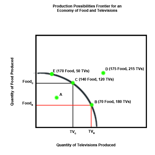